Harry Potter and the Half-Blood Prince

In Harry Potter and the Half-Blood Prince (2005), Dumbledore brings Harry along as he attempts to persuade Horace Slughorn to rejoin the Hogwarts faculty. Harry notices that Dumbledore’s right hand is shrivelled and blackened. During the school year, Dumbledore uses the Pensieve to teach Harry about Voldemort’s life and his rise to power. In one of the Pensieve visions, Harry witnesses Dumbledore’s first encounter with the young Tom Riddle. Dumbledore had known from the beginning that Riddle was dangerous, but believed that Hogwarts would change him. […]
1 Basic Markdown syntax
For the full list of supported document elements, please read the GFM spec. Below is a quick summary:
-
Headings start with a number of
#’s, e.g.,## level-two heading. -
Inline elements:
**strong**,_emphasis_,~~strikethrough~~,[text](link), and. -
Inline code is written in a pair of backticks, e.g.,
`code`. Code blocks can be indented, or fenced by```. -
List items start with
-,+, or*, e.g.,- item. A task list item is a regular list item with[ ]or[x]in the beginning, e.g.,- [ ] item. -
Block quotes start with
>. -
Tables are created with
|as the column separator (i.e., Pandoc’s pipe table).
2 Add-on features
In addition to GFM features, the litedown package also supports the following features.
2.1 Raw LaTeX/HTML blocks
Raw LaTeX and HTML blocks can be written as fenced code blocks with language
names =latex (or =tex) and =html, e.g.,
```{=tex}
This only appears in \LaTeX{} output.
```
Alert: possible infinite recursion!
2.2 LaTeX math
You can write both $inline$ and $$display$$ LaTeX math, e.g.,
\(\sin^{2}(\theta)+\cos^{2}(\theta) = 1\)
$$\bar{X} = \frac{1}{n} \sum_{i=1}^n X_i$$
$$|x| = \begin{cases} x &\text{if } x \geq 0 \\ -x &\text{if } x < 0 \end{cases}$$
2.3 Superscripts and subscripts
Write superscripts in ^text^ and subscripts in ~text~ (same syntax as
Pandoc’s Markdown), e.g., 210 and H2O.
2.4 Footnotes
Insert footnotes via [^n], where n is a footnote number (a unique
identifier). The footnote content should be defined in a separate block starting
with [^n]:. For example:
Insert a footnote here.[^1]

[^1]: This is the footnote.
2.5 Attributes
Attributes on images, links, fenced code blocks, and section headings can be
written in {}. For example, {.foo #bar width="50%"} will
generate an <img> tag with attributes in HTML output:
<img src="path" alt="text" id="bar" class="foo" width="50%" />
and ## Heading {#baz} will generate:
<h2 id="baz">Heading</h2>
For fenced code blocks, a special rule is that the first class name will be
treated as the language name for a block, and the class attribute of the
result <code> tag will have a language- prefix. For example, the following
code block
```{.foo .bar #my-code style="color: red;"}
```
will generate the HTML output below:
<pre>
  <code class="language-foo bar" id="my-code" style="color: red;">
  </code>
</pre>
2.6 Appendices
When a top-level heading has the attribute .appendix, the rest of the document
will be treated as the appendix. If section numbering is enabled, the appendix
section headings will be numbered differently.
2.7 Fenced Divs
A fenced Div can be written in ::: fences. Note that the opening fence must
have at least one attribute, such as the class name. For example:
::: foo
This is a fenced Div.
:::

::: {.foo}
The syntax `::: foo` is equivalent to `::: {.foo}`.
:::

::: {.foo #bar style="color: red;"}
This div has more attributes.

It will be red in HTML output.
:::
A fenced Div will be converted to <div> with attributes in HTML output,
e.g.,
<div class="foo" id="bar" style="color: red;">
</div>
For LaTeX output, it can be converted to a LaTeX environment if both the class
name and an attribute data-latex are present. For example,
::: {.tiny data-latex=""}
This is _tiny_ text.
:::
will be converted to:
\begin{tiny}
This is \emph{tiny} text.
\end{tiny}
2.8 Cross-references
To cross-reference an element, it must be numberd first. For section headings,
the numbers are automatically generated if the number_sections option is true.
For example, see 2.9.
For figures, these anchors are automatically generated if the chunk options
fig.cap (figure caption) or fig.env is not empty, e.g., the code chunk below
produces 1.
```{r}
#| nice-plot, fig.cap="OMG, I felt like crying when I drew this plot in Auckland! It has been almost two decades since I first learned R and knew this volcano.", fig.height=5
par(mar = c(4, 4, 1, .5))
filled.contour(volcano, color.palette = terrain.colors)
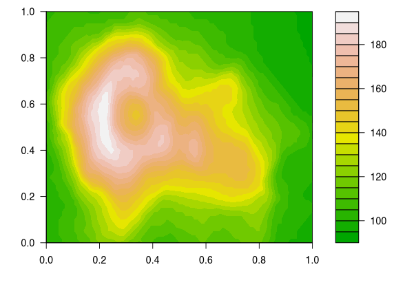
1 OMG, I felt like crying when I drew this plot in Auckland! It has been almost two decades since I first learned R and knew this volcano.
```
Similarly, you can reference tables, e.g., 1.
```{r}
#| nice-table, tab.cap="This is your familiar `mtcars` dataset. Note that data frames are printed to tables by default.", print.args=list(data.frame=list(limit=c(6, 10)))
mtcars
1
This is your familiar mtcars dataset. Note that data frames are printed to tables by default.
| mpg | cyl | disp | hp | … | gear | am | vs | qsec | wt | |
|---|---|---|---|---|---|---|---|---|---|---|
| Mazda RX4 | 21.0 | 6 | 160.0 | 110 | … | 4 | 1 | 0 | 16.46 | 2.620 |
| Mazda RX4 Wag | 21.0 | 6 | 160.0 | 110 | … | 4 | 1 | 0 | 17.02 | 2.875 |
| Datsun 710 | 22.8 | 4 | 108.0 | 93 | … | 4 | 1 | 1 | 18.61 | 2.320 |
| ⋮ | ⋮ | ⋮ | ⋮ | ⋮ | … | ⋮ | ⋮ | ⋮ | ⋮ | ⋮ |
| Ferrari Dino | 19.7 | 6 | 145.0 | 175 | … | 5 | 1 | 0 | 15.50 | 2.770 |
| Maserati Bora | 15.0 | 8 | 301.0 | 335 | … | 5 | 1 | 0 | 14.60 | 3.570 |
| Volvo 142E | 21.4 | 4 | 121.0 | 109 | … | 4 | 1 | 1 | 18.60 | 2.780 |
```
By default, tables are truncated to 10 rows (to avoid generating huge tables by accident), but this is configurable.
If you really want the “console output” for data frames, you can get it, too:
```{r}
#| print=xfun:::record_print.default
head(mtcars)
#>                    mpg cyl disp  hp drat    wt  qsec vs am gear carb
#> Mazda RX4         21.0   6  160 110 3.90 2.620 16.46  0  1    4    4
#> Mazda RX4 Wag     21.0   6  160 110 3.90 2.875 17.02  0  1    4    4
#> Datsun 710        22.8   4  108  93 3.85 2.320 18.61  1  1    4    1
#> Hornet 4 Drive    21.4   6  258 110 3.08 3.215 19.44  1  0    3    1
#> Hornet Sportabout 18.7   8  360 175 3.15 3.440 17.02  0  0    3    2
#> Valiant           18.1   6  225 105 2.76 3.460 20.22  1  0    3    1
```
2.9 Citations
This feature requires the R package rbibutils. Please make sure it is installed before using citations.
xfun::pkg_load2("rbibutils")
To insert citations, you have to first declare one or multiple bibliography databases in the YAML metadata, e.g.,
bibliography: ["papers.bib", "books.bib"]
Each .bib file contains entries that start with keywords. For example,
R-base is the keyword for the following entry:
@Manual{R-base,
  title = {R: A Language and Environment for Statistical Computing},
  author = {{R Core Team}},
  organization = {R Foundation for Statistical Computing},
  address = {Vienna, Austria},
  year = {2024},
  url = {https://www.R-project.org/},
}
Then you can use [@R-base] or @R-base to cite this item. You can include
multiple keywords in [ ] separated by semicolons.
2.10 Smart HTML entities
“Smart” HTML entities can be represented by ASCII characters, e.g., you can
write fractions in the form n/m. Below are some example entities:
1/2 |
1/3 |
2/3 |
7/8 |
1/7 |
1/9 |
1/10 |
(c) |
(r) |
(tm) |
|---|---|---|---|---|---|---|---|---|---|
| ½ | ⅓ | ⅔ | ⅞ | ⅐ | ⅑ | ⅒ | © | ® | ™ |
3 Code chunks and inline code
Global chunk options are controlled by litedown::reactor(), which is similar
to knitr::opts_chunk$set(), e.g.,
litedown::reactor(fig.width = 10, fig.height = 6)
Some quick examples:
litedown::mark('Hello _world_!')
<p>Hello <em>world</em>!</p>
litedown::mark('Hello _world_!', 'latex') # litedown does support latex output
Hello \emph{world}!
litedown::timing_data()
| source | line1 | line2 | label | time |
|---|---|---|---|---|
| 2024-ihaka-examples.Rmd | 205 | 209 | nice-plot | 0.049 |
| 2024-ihaka-examples.Rmd | 213 | 216 | nice-table | 0.004 |
| 2024-ihaka-examples.Rmd | 223 | 226 | chunk-4 | 0.002 |
| 2024-ihaka-examples.Rmd | 266 | 269 | smartypants | 0.002 |
| 2024-ihaka-examples.Rmd | 21 | 204 | 0.000 | |
| 2024-ihaka-examples.Rmd | 227 | 265 | 0.000 | |
| 2024-ihaka-examples.Rmd | 217 | 222 | 0.000 | |
| 2024-ihaka-examples.Rmd | 270 | 281 | 0.000 | |
| 2024-ihaka-examples.Rmd | 210 | 212 | 0.000 | |
| Total | 0.058 |
Inline R code expressions can have options, too, e.g.,
`{r, eval=FALSE, order=10} 1 + 1`.
4 Adding CSS/JS assets
Via meta variables in YAML:
output:
  litedown::html_format:
    meta:
      css: ["default", ...]
      js: [...]
All CSS/JS assets below are very lightweight and not tied to litedown (i.e., you can use them on any other web pages).
4.1 Article mode
css: ["@default", "@article"]
js: ["@sidenotes"]
Testing a footnote.1
Testing a full-width image:

4.2 Slides mode
css: ["@default", "@snap"]
js: ["@snap"]
-
Two modes: slides and article (depending on width and aspect ratio)
- You can’t have your cake and eat it too? That’s only true in Word and PowerPoint.
-
Keyboard shortcuts: f (fullscreen), o (overview), and m (mirror slides).
4.3 Tabsets
You can load the script tabsets.js and CSS tabsets.css to create tabsets
from bullet lists.
css: ["@tabsets"]
js: ["@tabsets"]
-
First tab
Hi, tab!
-
Second tab
This is the initial active tab.
-
Third tab
Bye, tab!
-
A child tabset
Content.
-
Another tab
More content
-
4.4 Code folding
js: ["@fold-details"]
4.5 Callout blocks
A callout block is a fenced Div with the class name callout-*. Callouts
require callout.css and callout.js:
css: ["@callout"]
js: ["@callout"]
For example:
This is a tip.
You can write arbitrary content, such as a blockquote.
Even another callout!
For the first time in your life, you have realized that you do not have to use fontawesome for icons!
Is that cool?
4.6 Right-align a quote footer
js: ["@right-quote"]
You can use the script
right-quote.jsto right-align a blockquote footer if it starts with an em-dash (---).—John Doe
4.7 Add anchor links to headings
css: ["@heading-anchor"]
js: ["@heading-anchor"]
4.8 Style keyboard shortcuts
css: ["@key-buttons"]
js: ["@key-buttons"]
Esc Tab Enter Space Delete Home End PrtScr PrintScreen
PageUp PageDown Up Down Left Right
Ctrl Control Shift Alt Cmd Command fn
Ctrl / Cmd + C
Ctrl / Cmd + Alt + I
Shift + Enter
Cmd + Shift + 9
fn + F
Alt + Click
4.9 HTML pagination
css: ["@pages"]
js: ["@pages"]
Press p for PDF, but that’s less fun than my Simon/Paul bots.
-
In the article mode, footnotes will be moved to the margin if
sidenotes.jsis used and the browser window is wide enough. ↩