15 Tips on Making Better Use of R Markdown

# 15 Tips on Making Better Use of R Markdown
### <a href="https://yihui.org">Yihui Xie</a>, RStudio
### 2019/11/15 @ DahShu

---

???

It always feels strange to do a webinar because you have to talk to a wall for an hour in an empty room... but I'm an introvert.

---

DahShu promoted this talk as if I were going to tell 15 jokes ("The joker Yihui, who unfortunately became a statistician, is going to introduce some awesome tips about R Markdown!"):

.center[![The title of DahShu's promotion article about this talk](https://user-images.githubusercontent.com/163582/68417998-05da4b80-015d-11ea-9153-f41cfcfb907c.png)]

(How about "learn one tip, get one joke for free"?)

???

This has put quite a bit pressure on me. It makes me feel if I fail to tell enough jokes in this talk, the organizers would never want to see me again. Anyway, this talk is mainly about R Markdown tips instead of jokes.

---
background-image: url(https://yihui.org/images/logo-tinytex.png)
background-position: top right
background-size: 18%

## 1. Why use TinyTeX?

- They are all too big: TeX Live, MiKTeX, MacTeX (~5Gb). TinyTeX ([yihui.org/tinytex](https://yihui.org/tinytex)) is ~150Mb when installed:

```r
    tinytex::install_tinytex()
    ```

- With the R function `tinytex::latexmk()`, two common LaTeX problems are automatically solved:

1. Missing LaTeX packages are automatically installed (doesn't require IT).
    2. The `.tex` document is compiled for the correct number of times to resolve cross-references (e.g., `pdflatex + bibtex + makeidx + pdflatex + pdflatex`).

- Demo: `01-tinytex.Rmd`

---
class: center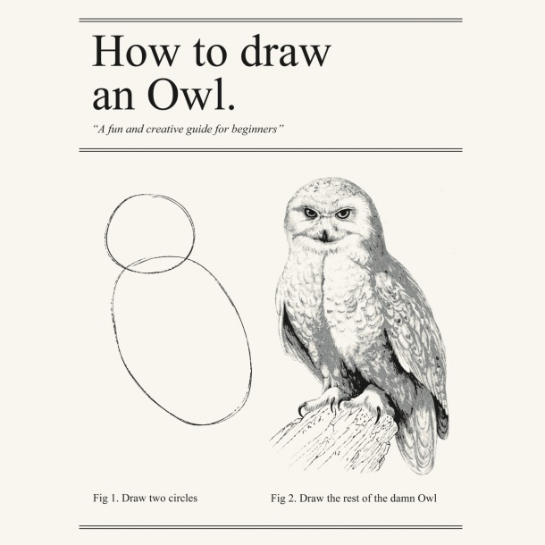

![How to draw an owl](gif/draw-an-owl.jpg)

???

Some of you may have seen this "fun and creative" guide to draw an owl. Sometimes it feels similar when you want to create a PDF. There are too many gory details for you to take care of.

---

![How to create a PDF](https://user-images.githubusercontent.com/163582/68422075-18f11980-0165-11ea-8589-24e168a3f246.jpg)

???

With TinyTeX and R Markdown, you just click the Knit button. Most intermediate steps are automated, and do not need your attention.

---

## 2. Generate a report from an R script

```r
#' Write your narratives after #'.
#' Of course, you can use **Markdown**.
#' Write R code in the usualy way.

1 + 1
str(iris)

#' Need chunk options? No problem.
#' Write them after #+, e.g.,

#+ fig.width=5
plot(cars)
```

- The script is converted to Rmd through `knitr::spin()`; then `rmarkdown::render()` will render the Rmd

- Demo: `02-spin.R` (either click the "Notebook" button in RStudio, or run `rmarkdown::render("02-spin.R")`)

---

[Some people](https://deanattali.com/2015/03/24/knitrs-best-hidden-gem-spin/) scream when they discover that an R script can play the same role as an R Markdown document...

.center[
![:image 45%, "The Scream"](https://www.edvardmunch.org/images/paintings/the-scream.jpg)
![:image 42.5%, "The Scream"](https://i.redd.it/294ep87hpcu31.jpg)
]

.right[images via [here](https://www.edvardmunch.org/the-scream.jsp) and [here](https://www.reddit.com/r/funny/comments/dm59b6/newsflash_the_scream_has_always_been_a_floppy/)]

???

This method is better for those who write more code than narratives. If you have a lot of narratives to write, I still recommend that you use R Markdown because otherwise you'd have to write a large amount of comments, which may feel awkward to read in an R script.

---

## 3. Convert Rmd to R script

Demo: `03-purl.Rmd`

```r
knitr::purl("03-purl.Rmd")  # output: 03-purl.R

# no documentation, pure code
knitr::purl("03-purl.Rmd", documentation = 0)

# full documentation in #' comments
knitr::purl("03-purl.Rmd", documentation = 2)
```

---

You just realized that all Rmd documents are actually R scripts wearing text masks.

---

## 4. Add citations

BibTeX databases:

```r
knitr::write_bib("base", file = "")
```

```
@Manual{R-base,
  title = {R: A Language and Environment for Statistical Computing},
  author = {{R Core Team}},
  organization = {R Foundation for Statistical Computing},
  address = {Vienna, Austria},
  year = {2019},
  url = {https://www.R-project.org/},
}
```

- Use `@key` to cite an entry (or `[@key]` if you need brackets, or cite multiple entries via `[@key-1; @key-2]`)

- Demo: `04-citation.Rmd`

---

## Please acknowledge your helpers

e.g., cite R packages that helped you

---

## 5. Cross-reference figures, tables, and sections

With the **bookdown** package (even if you are not writing a book), you can cross-reference things via `\@ref(key)`.

A few possible **bookdown** output formats:

```yaml
output:
  - bookdown::html_document2
  - bookdown::pdf_document2
  - bookdown::word_document2
```

Demo: `05-cross-reference.Rmd`

---

Cross-references are dynamically generated from their IDs, so you will never mistake "Figure 3" for "Figure 4" again.

---

## 6. Inline output of a character vector

```r
knitr::combine_words(c("apples", "oranges"))
## apples and oranges
knitr::combine_words(LETTERS[1:5])
## A, B, C, D, and E

# why not paste()?
paste(LETTERS[1:5], collapse = ", ")
## [1] "A, B, C, D, E"

knitr::combine_words(c("hook", "line", "sinker"))
## hook, line, and sinker
knitr::combine_words(c("the rhinos", "Washington", 
    "Lincoln"))
## the rhinos, Washington, and Lincoln
```

Demo: `06-combine.Rmd`

---

## The importance of the Oxford Comma

[via](https://knowyourmeme.com/photos/946417-oxford-comma)

---

## 7. Line breaks (not paragraphs)

This may sound like a simple question, but I guess most people don't know the answer: how to break a line in the output? In LaTeX, you use `\\`; in HTML, you use `<br/>`. In Markdown, what do you use? By default, simply a line break in source won't work (it will be ignored).

The answer is  
add _two trailing spaces_ before you break a line in the source.

Demo: `07-quote.Rmd`, using the **blogdown** addin "Quote Poem" in RStudio to add these trailing spaces when you quote a large amount of text and want to preserve the line breaks (such as in poems or lyrics).

---

Sometimes a simple task can drive you crazy...

When in doubt, read the manual: https://pandoc.org

---

## 8. Put all code in the appendix

- The key: the chunk option `ref.label` to reference other code chunks.

- More info: https://yihui.org/en/2018/09/code-appendix/

- Demo: `08-code-appendix.Rmd`

---

You can move your code freely in an Rmd document using `ref.label`, _without cut-and-paste_.

---

## 9. [Create an animation](https://yihui.org/en/2018/08/gifski-knitr/)

To create a GIF animation from all R plots in a code chunk, install the **gifski** package. Then use the chunk option `animation.hook='gifski'`:

````md
```{r, animation.hook='gifski'}
for (i in 1:2) {
  pie(c(i %% 2, 6), col = c('red', 'yellow'), labels = NA)
}
```
````

.center[![:image 45%, "Pacman"](https://user-images.githubusercontent.com/163582/44246516-30c93000-a1a4-11e8-8aa5-8876e51a227f.gif)]

---

Enjoy your animations!

---

## 10. Cache time-consuming code chunks

Use the chunk option `cache = TRUE` if a code chunk is time-consuming and the code doesn't change often.

---

No free lunch. Simple tricks can have costs, too ([more here](https://yihui.org/en/2018/06/cache-invalidation/)).

---

## 11. Add logos to your R plots

The key: the chunk option `fig.process` can be a function to post-process your plots.

````md
```{r, fig.process=function(x, options) { x }}
# plot
```
````

Demo: `11-magick.Rmd`

---
class: center

## `fig.process` == Strong force

![:image 60%, Feel the force](gif/git-push-force.gif)

Be creative. Use your imagination.

---

## 12. Add real LaTeX math expressions to R plots

- You may know `?plotmath`, but these tricks in base R graphics do not produce real LaTeX math expressions
    
    ```r
    plot(cars, main = expression(hat(beta) == (X^t * X)^{-1} * X^t * y))
    ```

- The (perhaps only) R package that allows you to write LaTeX expressions in R plots is **tikzDevice**.

- How to use **tikzDevice** in R Markdown? Short answer: use the chunk option `dev = "tikz"`. But...

- Demo: `12-tikz.Rmd`

---

You definitely need some skills to create beautiful math expressions in R plots...

![:image 100%, "You need some skills to write beautiful LaTeX math"](gif/cool-car.gif)

---

## 13. Use other languages

- Python, Julia, SQL, C++, shell scripts, JavaScript, CSS, ...

- To know all languages supported in **knitr** (there are more than 40): `names(knitr::knit_engines$get())`

````md
    ```{python}
    x = 42
    ```
    ````

- Demo: `13-lang.Rmd`

---

Code chunks of all different languages worked perfectly...

???

In an R Markdown document, R works, Python works, Julia works, C++ works, ... Yeah!

---

## 14. Child documents

You can split your long documents into shorter ones, and include the shorter documents as child documents, e.g.,

````md
```{r, child='analysis.Rmd'}
```

```{r, child=c('one.Rmd', 'another.Rmd')}
```
````

---

You can have as many happy child documents as you want...

---

## 15. Start bookdown and blogdown projects

In RStudio: `File -> New Project -> New Directory`; select "Book" or "Website" projects.

---

Write a book? Create a website? Sounds scary...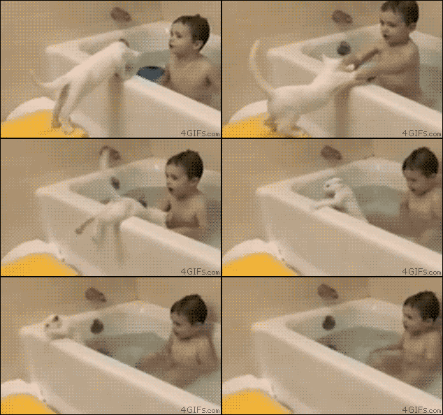

---
class: inverse

## More fun with R Markdown

R Markdown + Shiny (+ JavaScript): https://yihui.shinyapps.io/face-pi/

---
class: center, middle

# Thank you!

## Slides: https://bit.ly/dahshu-down

Examples can be downloaded at: https://bit.ly/dahshu-demo

### Contact info: https://yihui.org/en/about/#contact-me